Multiple measures compared by land type

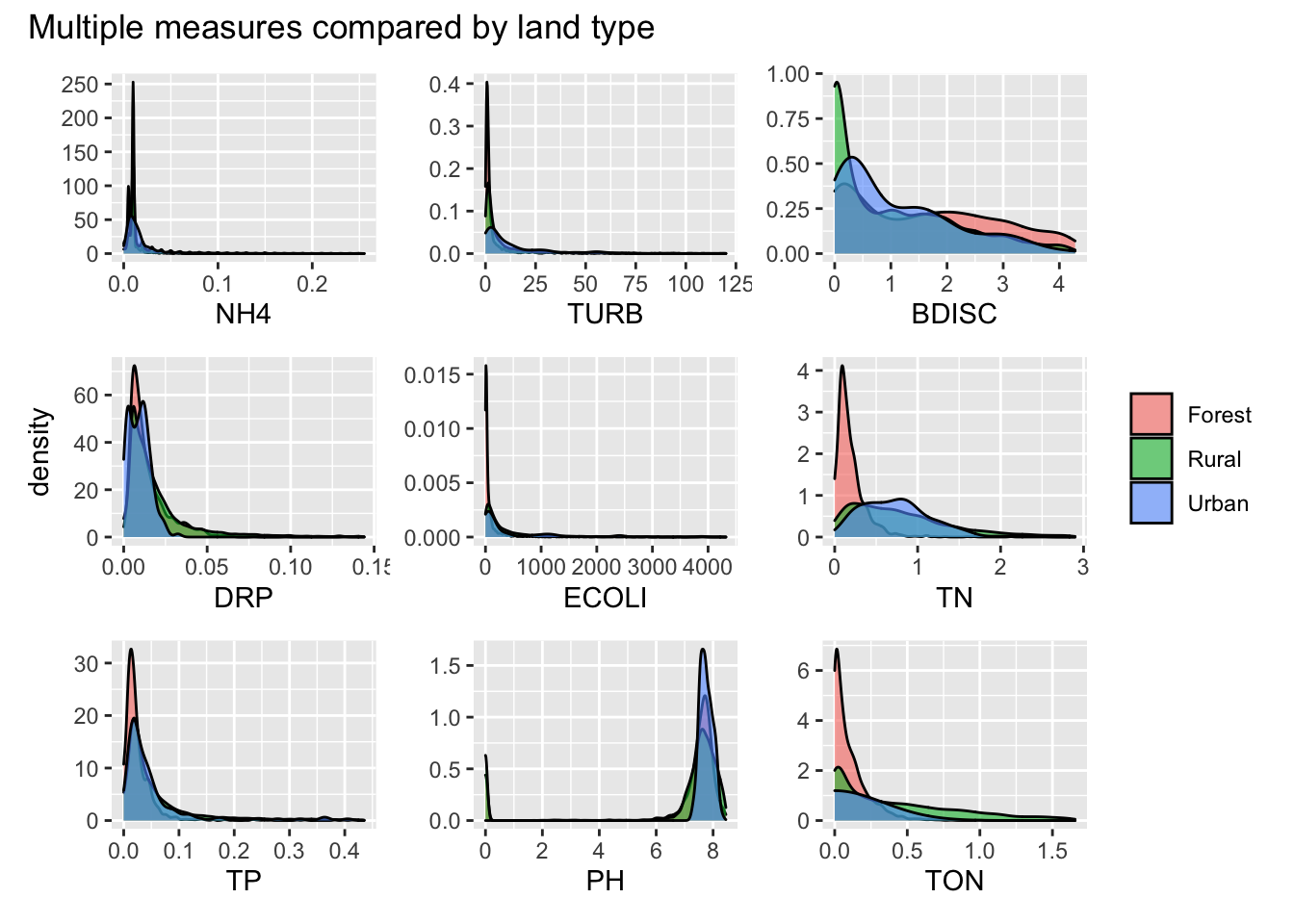
I chose this data story because it was one of the suggested ones and seemed easy enough to represent. I’ve chosen density plots as they show the density of data and help a user to understand if there are any differences in the data based on the land type. As shown most measures have similar densities regardless of the land type except for nitrogen (TN and TPON) and BDISC(Water Clarity)

library(tidyverse)
library(patchwork)

lawa <- read_csv("http://www.massey.ac.nz/~jcmarsha/161122/LAWA/lawa41.csv")

AllLand <- lawa %>% select(SWQLanduse, NH4, TURB, BDISC, DRP, ECOLI, TN, TP, PH, TON)

# Changed NaN values to 0 otherwise the graphs are ruined by outliers
AllLand[is.na(AllLand)] <- 0

NH4Trim <- AllLand %>% filter(NH4 < quantile(NH4,0.95))
TURBTrim <- AllLand %>% filter(TURB < quantile(TURB,0.95))
BDISCTrim <- AllLand %>% filter(BDISC < quantile(BDISC,0.95))
DRPTrim <- AllLand %>% filter(DRP < quantile(DRP,0.95))
ECOLITrim <- AllLand %>% filter(ECOLI < quantile(ECOLI,0.95))
TNTrim <- AllLand %>% filter(TN < quantile(TN,0.95))
TPTrim <- AllLand %>% filter(TP < quantile(TP,0.95))
PHTrim <- AllLand %>% filter(PH < quantile(PH,0.95))
TONTrim <- AllLand %>% filter(TON < quantile(TON,0.95))

# Function for reuse in multiple plots
fixTheme <- function() {
  theme(legend.position="none",axis.title.y = element_blank())
}

NH4Plot <- ggplot(NH4Trim) +
  geom_density(mapping=aes(x=NH4, fill=SWQLanduse), alpha=0.6) + fixTheme()
TURBPlot <- ggplot(TURBTrim) +
  geom_density(mapping=aes(x=TURB, fill=SWQLanduse), alpha=0.6) + fixTheme()
BDISCPlot <- ggplot(BDISCTrim) +
  geom_density(mapping=aes(x=BDISC, fill=SWQLanduse), alpha=0.6) + fixTheme()
DRPPlot <- ggplot(DRPTrim) +
  geom_density(mapping=aes(x=DRP, fill=SWQLanduse), alpha=0.6) + theme(legend.position = "none")
ECOLIPlot <- ggplot(ECOLITrim) +
  geom_density(mapping=aes(x=ECOLI, fill=SWQLanduse), alpha=0.6) + fixTheme()
TNPlot <- ggplot(TNTrim) +
  geom_density(mapping=aes(x=TN, fill=SWQLanduse), alpha=0.6) + theme(legend.title = element_blank(), axis.title.y = element_blank())
TPPlot <- ggplot(TPTrim) +
  geom_density(mapping=aes(x=TP, fill=SWQLanduse), alpha=0.6) + fixTheme()
PHPlot <- ggplot(PHTrim) +
  geom_density(mapping=aes(x=PH, fill=SWQLanduse), alpha=0.6) + fixTheme()
TONPlot <- ggplot(TONTrim) +
  geom_density(mapping=aes(x=TON, fill=SWQLanduse), alpha=0.6) + fixTheme()

NH4Plot + TURBPlot + BDISCPlot + DRPPlot + ECOLIPlot + TNPlot + TPPlot + PHPlot + TONPlot + plot_annotation(title="Multiple measures compared by land type")