A3.2
Write a paragraph describing your data story (e.g. why you chose the story and chart types, and what it shows) below.
Much of New Zealand Aoteaora’s economy is derived from agriculture and forestry, also NZ presents a very typical topography: hills, rivers, and mountains. Water in NZ aoteaora is present everywhere, therefore for these reasons I have decided to analyse water quality and to focus on relationship between topography, land use and water quality. According to Stats NZ, in 2007, farmland alone represented 54.8% of the total New Zealand land area, whereas forestry was 8%.
I have chosen two water contaminants indicators for this study: 1) Total Nitrogen (TN): TN was chosen to study Nitrogen contaminant, instead of Ammoniacal nitrogen (NH4) and Total Oxygenated Nitrogen (TON), to analyse TN water contamination trend over the years in Forest, Rural or Urban land. 2) E.coli was chosen as a faecal indicator. I have decided to plot only 2 indicators out of the 9 given in order to have a final clear plot. Also it is also worth mentioning that TON,TN, and NH4 are three indicators measuring nitrogen contamination. I have chosen TN, because it measures most forms of nitrogen in water. I have chosen E.coli as an indicator bacteria for this plot. Nitrogen in water comes from fertiliser, wastewater, treatment plants , industrial and chemical wastes. E.coli water contamination occurs if the soil is contaminated with E.coli.
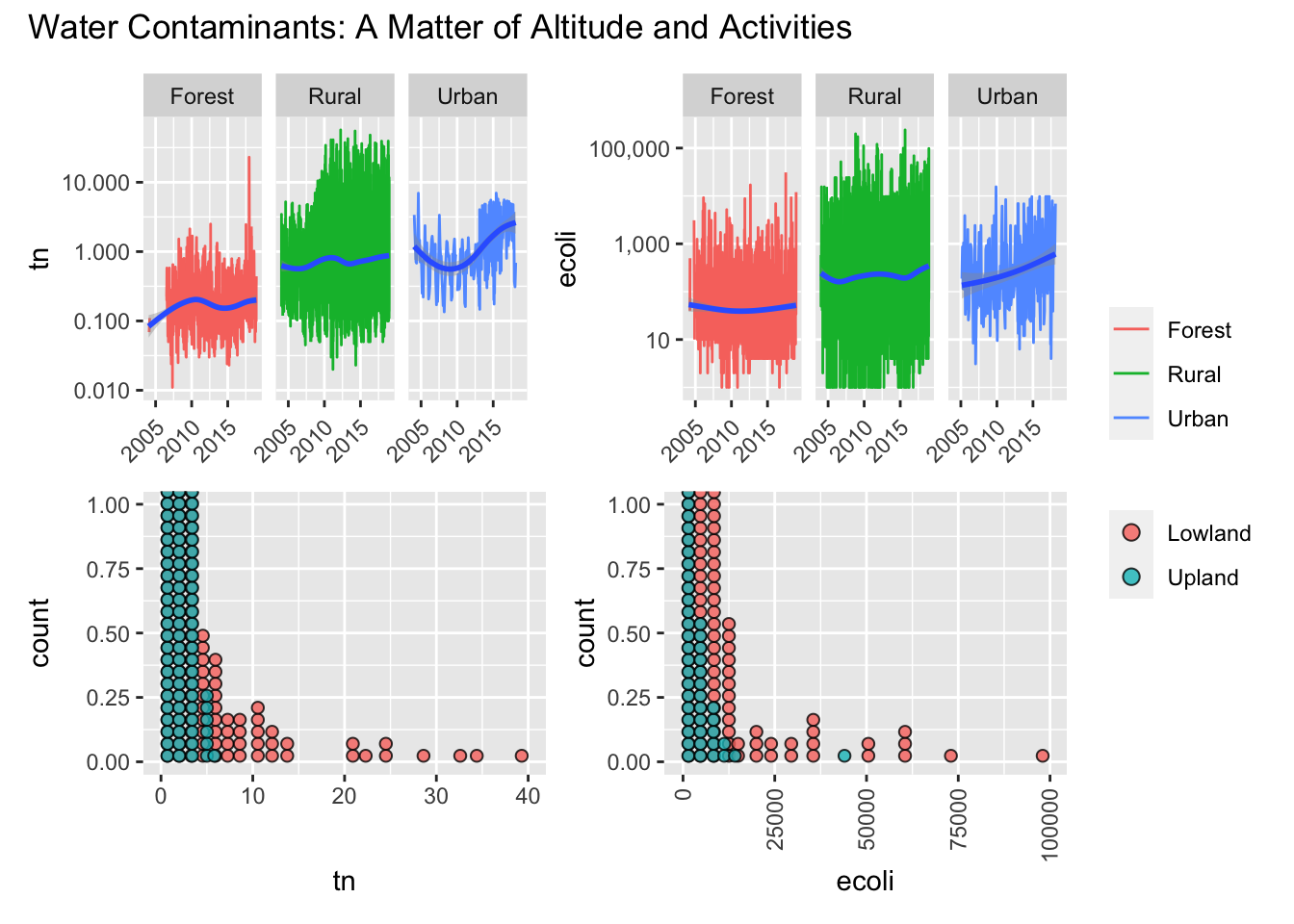
On the first plot, nitrogen detection level is higher in rural and urban water, than in forest water. The first mini graph shows that for the forest water, the nitrogen level trend is increasing from 2004 until 2015. From 2004 until 2010, the nitrogen level increases from a log factor of 0.1 to 0.5, and stays at the same level until 2015 In rural water, the nitrogen level trend is increasing slightly from 2004 until 2015. The nitrogen detection level is 10 times higher in rural water than in the forest water. From 2004 until 2010, the nitrogen detection level increases from 0.9 to 1, then it decreases a little from 2010, to increase again until 2015 and to reach 1. The third mini graph shows that in urban water the nitrogen level trend is increasing. From 2005 until 2007 the level detection of TN goes down from 1 to 0.7, whereas from 2007 until 2015 it increases over 1.
The second plot shows that the E.coli contamination is lower in forest water than in rural and urban waters. In Forest water, from 2004 until 2015, the E.coli detection level is stagnant,1. In rural water, the bacteria detection is higher, than in forest water, and the level is also constant from 2004 until 2015. The Nitrogen urban trend is interesting, in 2015 the detection level in urban water is less than in rural water, and it then increases from 2005 until 2015. In 2015, the level of detection of nitrogen in urban water is higher than in urban area, and it nearly reaches 1000 on the log scale. It is also worth mentioning that data for urban water are less than data for rural or forest water in both plots, for E.coli or TN detection. The higher level of nitrogen detection in rural and urban area can be explained by the use of fertiliser and industrial waste, respectively. The high level of E.coli detection in rural area can be explained by the animals waste contaminating the rural land, whereas in the urban area it can be explained by leakage of sewer systems.
The last plots compares the level of TN and E.coli in upland or lowland. It shows that there is a low level of detection of E.coli and TN in upper land, but a high level of detection of TN and E.coli in lowerland. This data could be explained by the fact that most farms are on lowerland. Also it is worth mentioning that the water upland will drain and accumulate in the lower land, and therefore maybe also contribute to a higher level of detection in the lower land for E.coli and TN.
library(tidyverse)
library(janitor)
library(lubridate)
library(patchwork)

lawa <- read_csv("http://www.massey.ac.nz/~jcmarsha/161122/LAWA/lawa42.csv")
lawa%>%clean_names()->lawa_cleaned

lawa_cleaned %>% filter(swq_landuse %in% c("Rural","Forest","Urban"))-> three_use

three_use%>%ggplot()+geom_line(mapping = aes(x=date,y=tn,col=swq_landuse))+geom_smooth(mapping=aes(x=date,y=tn))+scale_y_log10(labels=scales::label_comma())+ facet_wrap(vars(swq_landuse))+labs(col=NULL)+theme(axis.text.x = element_text(angle = 45, vjust = 0.9, hjust=1))+theme(axis.title.x=element_blank())-> p1

three_use%>%ggplot()+geom_line(mapping = aes(x=date,y=drp,col=swq_landuse))+geom_smooth(mapping=aes(x=date,y=drp))+scale_y_log10(labels=scales::label_comma())+facet_wrap(vars(swq_landuse))+labs(col=NULL)-> p2

three_use%>%ggplot()+geom_line(mapping = aes(x=date,y=ecoli,col=swq_landuse))+geom_smooth(mapping=aes(x=date,y=ecoli))+scale_y_log10(labels=scales::label_comma())+facet_wrap(vars(swq_landuse))+labs(col=NULL)+theme(axis.text.x = element_text(angle = 45, vjust = 0.9, hjust=1))+theme(axis.title.x=element_blank())->p3

three_use%>%ggplot()+geom_line(mapping = aes(x=date,y=bdisc,col=swq_landuse))+geom_smooth(mapping=aes(x=date,y=bdisc))+scale_y_log10(labels=scales::label_comma())+facet_wrap(vars(swq_landuse))+labs(col=NULL)->p4


lawa_cleaned%>%mutate(Year = year (date)) %>% filter(Year == 2018)%>%ggplot()+geom_dotplot(mapping=aes(x=tn, fill=swq_altitude),alpha=0.8)+labs(fill=NULL)->t1

lawa_cleaned%>%mutate(Year = year (date)) %>% filter(Year == 2018)%>%ggplot()+geom_dotplot(mapping=aes(x=ecoli, fill=swq_altitude),alpha=0.8)+labs(fill=NULL)+theme(axis.text.x = element_text(angle = 90, vjust = 0.5, hjust=1))->t2

lawa_cleaned%>%mutate(Year = year (date)) %>% filter(Year == 2018)%>%ggplot()+geom_dotplot(mapping=aes(x=ph, fill=swq_altitude),alpha=0.8)+labs(fill=NULL)->t3

lawa_cleaned%>%mutate(Year = year (date)) %>% filter(Year == 2018)%>%ggplot()+geom_dotplot(mapping=aes(x=ecoli, fill=swq_altitude),alpha=0.4)+labs(fill=NULL)->t4

(p1 | p3 )/(t1|t2)+plot_layout(guides = 'collect')+plot_annotation(title="Water Contaminants: A Matter of Altitude and Activities")