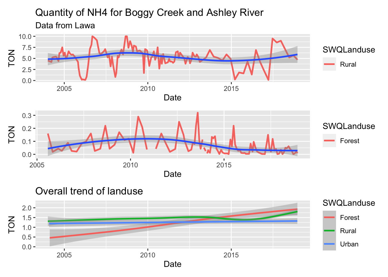
The story that I have decided portray with this data set, is the change in Oxygenated Nitrogen (TON) quantity over time (Date). The reason I chose this data set to compare, is due to the importance of this chemical for life on earth. Approximately 80% of the earth’s atmosphere is nitrogen, and provides essential nutrients needed for plant growth, as well as a major chemical component to many biological macromolecules such as proteins (Amino acids) and DNA (Nucleic Acids). However, nitrogen in an oxidised state, is truly harmful to humans (in large doses) and even more dangerous to wildlife, in particular stream/river/creek ecological systems. With this in mind, I believe that my graphical representation of the “lawa” dataset provides a viewer with the insight to the potential causes for Oxygenated Nitrogen (NO2) contamination in local NZ water systems.
The conclusion that I have drawn, is that Rural landuse contributes to a far higher amount of NO2 when compared to other landuses, such as Urban or Forest. After research into NO2 sources from the lawa website, I found that the reason for this is due to the process of denitrification from farm stock waste. Whereby microbially facilitated processes produce NO2. Also, I found that farmers tend to use nitrogen rich fertilizers, that when not properly maintained, can lead to a significant increase in NO2 concentration in neighboring waterways, due to rain washing it away. However, what I did find interesting was that when I made a rough indication of an overall trend for my third graph, I used all the data from the dataset “lawa” and found that urban landuse has been consistent throughout the timeperiod recorded, whereas rural had slowly increased. Interestingly, it seemed Forest landuse has a positive trend, increasing in TON over time, indicating more research required in this landuse.
library(tidyverse)
library(patchwork)

lawa <- read_csv("http://www.massey.ac.nz/~jcmarsha/161122/LAWA/lawa79.csv")

boggy_creek <- lawa %>% filter(SiteID == "boggy creek u/s lake road")

ashley_river <- lawa %>% filter(SiteID == "ashley river u/s ashley gorge rd")


g1 = ggplot(boggy_creek) +
  geom_line(aes(x= Date, y= TON, col = SWQLanduse), size = 1) +
  geom_smooth(aes(x= Date, y= TON))+

labs(
    title = "Quantity of NH4 for Boggy Creek and Ashley River",
    subtitle = "Data from Lawa"
  )

g2 = ggplot(ashley_river) +
  geom_line(aes(x= Date, y= TON, col = SWQLanduse), size = 1) +
  geom_smooth(aes(x= Date, y= TON))

g3 = ggplot(lawa) +
  geom_smooth(aes(x= Date, y= TON, col = SWQLanduse)) +
  labs(
    title = "Overall trend of landuse")

g1 / g2 / g3