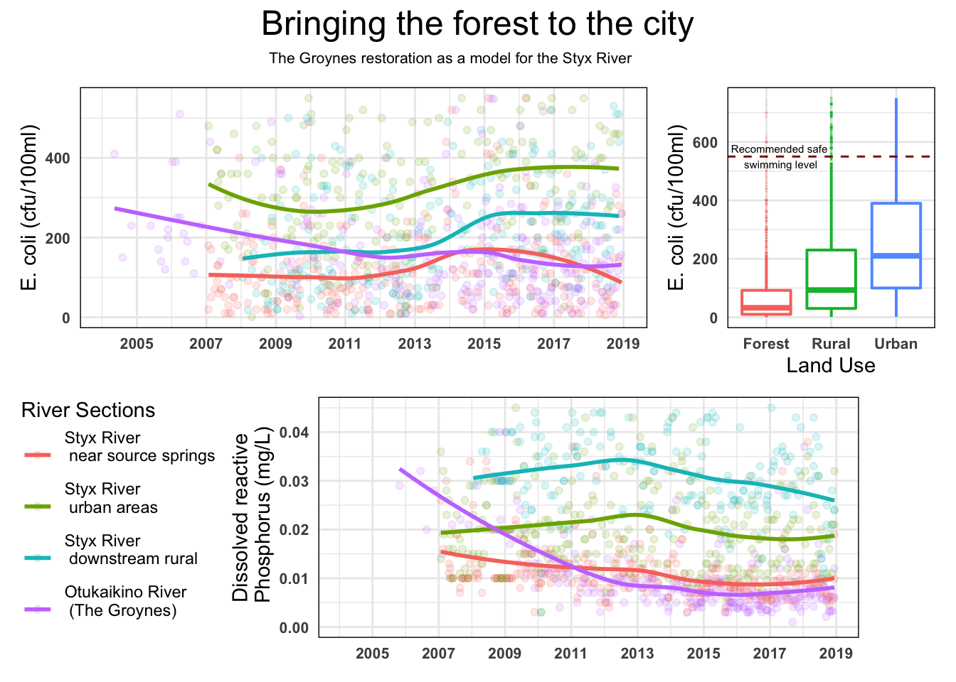
The water quality measures, especially in E. coli, between the urban, rural and forest land use show results that may be against the current public perception of rural / urban water quality. Considering the ambition to plant 1 billion trees, targeting some of that project towards riparian planting in urban areas may assist in improving water quality.
There is currently large amount of development in the Styx River catchment area, although a small catchment it begins with small springs, runs through an urban area with other urban stream inflows,then travels through a rural area of cropping and pasture. Areas of the catchment, especially around developing urban areas are seeing increasing riparian planting and some wetland restoration.
As a point of comparison the Otukaikino River in the catchment immediately northwest has had extensive planting and ecological restoration over the last 20 years. The improvements seen in this river show a picture of what may be achievable with ecological restoration along the Styx.
library(tidyverse)
library(stringr)
library(patchwork)

lawa <- read_csv("http://www.massey.ac.nz/~jcmarsha/161122/LAWA/lawa62.csv")
# A comparison of Styx River and Otukaikino River (The Groynes)

# Data groups
groynes_data <- lawa %>%
  filter(str_detect(SiteID, "otukaikino")) %>%
  mutate(cat = "Otukaikino River                  \n (The Groynes)\n")

styx_source_data <- lawa %>%
  filter(str_detect(SiteID, "styx river at gardiners road") |
  str_detect(SiteID, "smacks creek at gardiners road")) %>%
  mutate(cat = "Styx River\n near source springs\n")

styx_urban_data <- lawa %>%
  filter(str_detect(SiteID, "styx river at main north road") |
  str_detect(SiteID, "styx river at marshland road bridge")) %>%
  mutate(cat = "Styx River\n urban areas\n")

styx_downstream_data <- lawa %>%
  filter(str_detect(SiteID, "styx river at richards bridge") |
  str_detect(SiteID, "styx river at harbour road bridge")) %>%
  mutate(cat = "Styx River\n downstream rural\n")

dframe <- rbind(groynes_data, styx_source_data, styx_urban_data, styx_downstream_data)
legend_list <- c("Styx River\n near source springs\n", "Styx River\n urban areas\n",
                 "Styx River\n downstream rural\n",
                 "Otukaikino River                  \n (The Groynes)\n")

# Plot 1 lower plot
p1 <- ggplot(dframe, aes(x = Date, y = DRP, colour = fct_relevel(cat, legend_list))) +
  geom_point(alpha = 0.15) +
  geom_smooth(se = FALSE) +
  scale_y_continuous(limits = c(0,0.045)) +
  scale_x_date(date_breaks = "2 years", date_labels = "%Y") +
  labs(y = "Dissolved reactive\n Phosphorus (mg/L)", x = NULL) +
  theme_minimal() +
  theme(legend.position = "none",
        axis.text = element_text(face = "bold", size = 8),
        panel.border = element_rect(fill = NA))

# Plot 2 top left plot
p2 <- ggplot(dframe, aes(x = Date, y = ECOLI, colour = fct_relevel(cat, legend_list))) +
  geom_point(alpha = 0.15) +
  geom_smooth(se = FALSE) +
  scale_y_continuous(limits = c(0,550)) +
  scale_x_date(date_breaks = "2 years", date_labels = "%Y") +
  labs(colour = "River Sections",
       y = "E. coli (cfu/100ml)",
       x = NULL) +
  theme_minimal() +
  theme(axis.text = element_text(face = "bold", size = 8),
        panel.border = element_rect(fill = NA))

# Plot 3 top right - box plot
p3 <- lawa %>%
  filter(!is.na(ECOLI)) %>%
  group_by(SWQLanduse) %>%
  ggplot(aes(x = SWQLanduse, y = ECOLI, col = SWQLanduse)) +
    geom_boxplot(outlier.alpha = 0.1, outlier.size = 0.01, outlier.shape = 4, size = 0.7) +
    scale_y_continuous(limits = c(0, 750)) +
    geom_hline(yintercept = 550, colour = "darkred", linetype = "dashed") +
    annotate("text", x = 1.2, y = 550,
           label = "Recommended safe\n swimming level",
           size = 2) +
    labs(y = "E. coli (cfu/100ml)", x = "Land Use") +
    theme_minimal() +
    theme(legend.position = "none",
          axis.text = element_text(face = "bold", size = 8),
          panel.border = element_rect(fill = NA))


# patchwork
plot_full <- p2 + p3 + guide_area() + p1

plot_layout <- c(area(t=1, l=1, b=1, r=7),
                  area(t=1, l=8, b=1, r=10),
                  area(t=2, l=1, b=2, r=2),
                  area(t=2, l=3, b=2, r=9))

#plot(plot_layout)
plot_full + plot_layout(guides = "collect", design = plot_layout) +
  plot_annotation(title = "Bringing the forest to the city",
                  subtitle = "The Groynes restoration as a model for the Styx River",
                  theme = theme(plot.title = element_text(size = 18, hjust = 0.5),
                                plot.subtitle = element_text(size = 8, hjust = 0.45)))