As Hamanatua Stream becomes basic, Waimata River becomes acidic

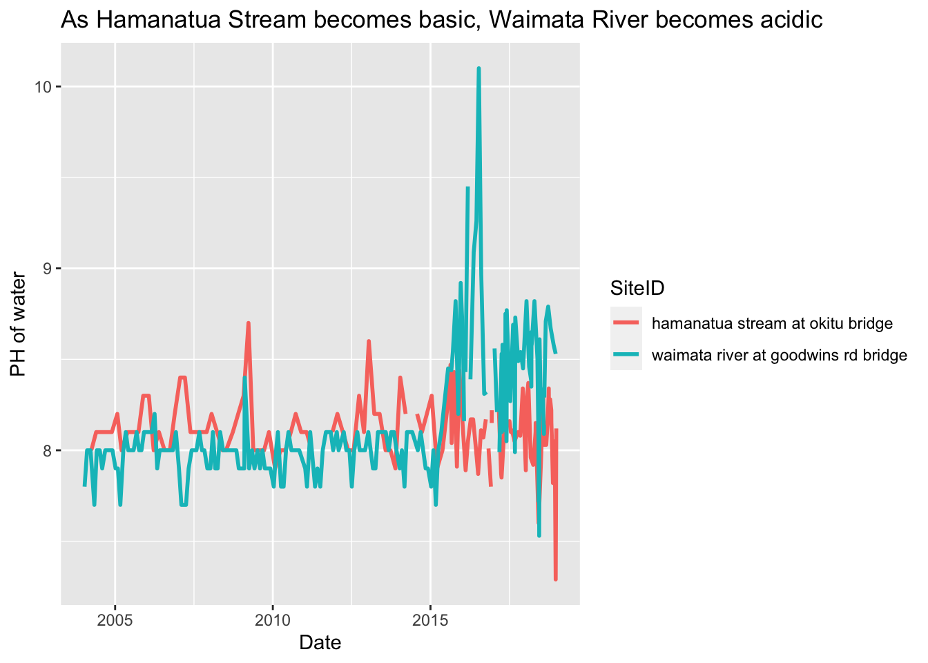
I chose this story to show the difference between the PH’s of Hamanatua stream & Waimata river, I picked them due to the fact they were very similar before 2015, but after 2015 something has happened which has caused an influence to both of them. I’ve used line graphs to show the data, as it allows the viewer to see the detail between the two without them interrupting each other, I’ve used colour to distinguish between the two sites. The graph shows how after 2015, something happened which had an impact on the PH of these two sites. Interestingly, Hamanatua stream has had a decline in PH towards seven, whereas the Waimata river has had a sharp jump towards ten before equalizing at approximately 9.75 on the PH scale.

library(tidyverse)

lawa <- read_csv("http://www.massey.ac.nz/~jcmarsha/161122/LAWA/lawa36.csv")

average_ph <- lawa %>% group_by(SiteID, Date, PH) %>% select(SiteID, Date, PH) %>% filter(SiteID == "waimata river at goodwins rd bridge" | SiteID == "hamanatua stream at okitu bridge")

ggplot(average_ph) + geom_line(mapping=aes(x=Date, y=PH, color=SiteID), size = 1) + labs(x = "Date", y = "PH of water", title = "As Hamanatua Stream becomes basic, Waimata River becomes acidic")