Are Falling PH Levels a concern?

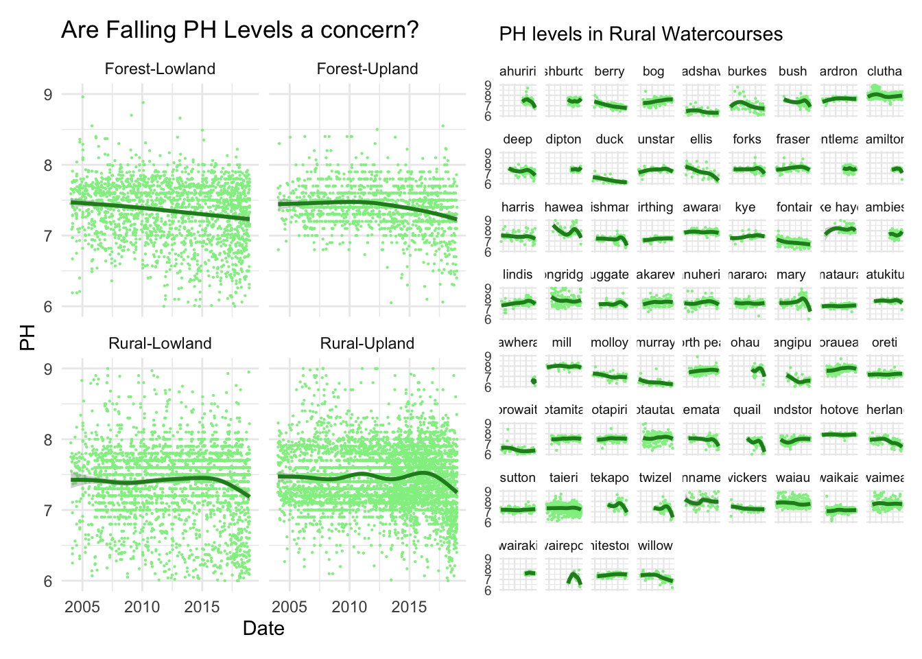
A cursory examination of the data showed a surprisingly strong drop in PH levels over the last five years. Splitting the data up by land use showed that these changes were concentrated in rural areas. I decided to use geom_point and geom_line functions to track this drop as I wanted to be able to show both the trend over time and the individual datapoints. On the left I’ve split the data up by broad biome. Rural areas, presumably including farmland, appear to bear the bulk of the PH change. The graphs on the right show the Rural streams and rivers represented in the data. Some of these watercourses are stable and some show, often rapidly, declining PH levels, many of these initially having grown more alkali. A sudden increase in alkalinity in watercourses can trigger a reaction and reversal often leaving the watercourse more base then before the spike. This could be part of the cause of the drop in PH since 2015.

library(tidyverse)
library(patchwork)
library(magrittr)  

lawa <- read_csv("http://www.massey.ac.nz/~jcmarsha/161122/LAWA/lawa93.csv")

Blockdata <- lawa%>%
  unite( "Location", SWQLanduse:SWQAltitude, sep = "-", remove = TRUE)%>%
  group_by(Location)

RuralRivers <- lawa%>%
  filter(SWQLanduse=="Rural", PH!="NA")%>%
  unite( "Location", SWQLanduse:SWQAltitude, sep = "-", remove = TRUE)%>%  
  mutate(across(.cols = SiteID, .fns = tolower))%>%
  separate(SiteID, c("Site1", NA), sep = " river")%>%
  separate(Site1, c("Site2", NA), sep = " stream")%>%
  separate(Site2, c("Site3", NA), sep = " stm")%>%
  separate(Site3, c("Site4", NA), sep = " rv")%>%
  separate(Site4, c("Site5", NA), sep = " ck")%>%
  separate(Site5, c("Site6", NA), sep = "quailburn road")%>%
  separate(Site6, c("Site7", NA), sep = " at ")%>%
  separate(Site7, c("Site8", NA), sep = "creek")%>%
  separate(Site8, c("Site9", NA), sep = " d/s")%>%
  separate(Site9, c("Site10", NA), sep = "canal")%>%
  separate(Site10, c("Site11", NA), sep = "burn")%>%
  separate(Site11, c("Site", NA), sep = "smith")%>%
  filter(Site!="page")%>%
  group_by(Location)%>%
  select(Location, PH, Date, Site)

p1 <- ggplot(Blockdata)+
  theme_minimal()+
  geom_point(mapping=aes(y=PH, x=Date), colour =  "light green", size=0.1)+
  geom_smooth(mapping=aes(y=PH, x= Date),colour =  "forest green")+
  ylim(6,9)+
  facet_wrap(vars ( Location))

 p2 <- ggplot(RuralRivers)+
  theme_minimal(base_size = 9)+
  geom_point(mapping=aes(y=PH, x=Date), colour =  "light green", size=0.1)+
  geom_smooth(mapping=aes(y=PH, x= Date),colour =  "forest green")+
  theme(axis.text.x=element_blank(), axis.title.x = element_blank(), axis.title.y = element_blank())+
  ylim(6,9)+
  facet_wrap(vars(Site))

p1+ ggtitle("Are Falling PH Levels a concern?")+p2 + ggtitle("PH levels in Rural Watercourses")