Chapter 1 Introduction
1.1 What is Data Mining?
What is data mining, and how does it differ from the statistics? It’s difficult (or perhaps we should say impossible) to give a definitive answer to those questions. The boundaries between statistics, data mining and machine learning are ill defined, and you would likely get different answers from a computer scientist and a statistician if asked to map out the territories of the respective disciplines.
In this paper you will get a statistician’s take on data mining. We regard data mining as essentially statistical in nature, albeit with a different slant to many other statistics courses that you may encounter at university. We’ll try to give you a flavour of how data mining differs from mainstream classical statistics through a couple of examples.
Example 1.1 Weight gain in goats
This example concerns a designed experiment (conducted in Lincoln, New
Zealand) to investigate the effect of different drenching regimes on
goats. Goats are drenched as a matter of course to prevent worm
infestation, but it was conjectured that the standard method of
drenching was insufficient. A total of 40 goats were divided at random
into two groups of 20. Each goat was weighed at the start of the year,
and then again at the end of the year. Groups in the first group were
treated using a standard drenching program, while those in the second
underwent an intensive drenching regimen (involving more frequent
drenches through the year). The variables recorded in the dataset
goats are initial weight,
weight gain through the year (both measured in kilograms), and treatment
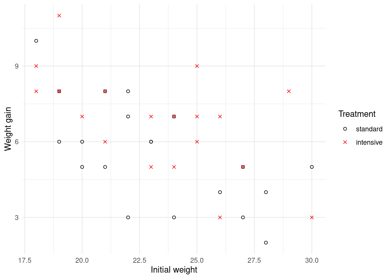
(either standard or intensive drenching). The data are plotted in Figure
1.1 below.

Figure 1.1: Scatterplot of weight gain against initial weight for goats on standard and intensive drenching regimens.
The principal question of interest here is whether or not the type of drenching program affects a goat’s weight gain. A secondary question is whether the level of weight gain depends on the goat’s initial weight, and if so in what way.
We are definitely in the realm of classical statistics here! It is the kind of dataset and scientific problem that would have been familiar Ronald Fisher and Karl Pearson as they developed the basic theory and methods for modern statistics, almost a century ago1. The dataset is of modest size, with \(n=40\) cases and \(p=3\) variables (namely weight gain; initial weight; and treatment program). Moreover, the analysis of these data should be driven by the specific scientific questions just discussed. A statistician would use standard tools like regression and hypothesis testing2. The statistical models used will be easy to interpret, with model parameters likely to have some clear physical meaning.
Example 1.2 Amazon reviews
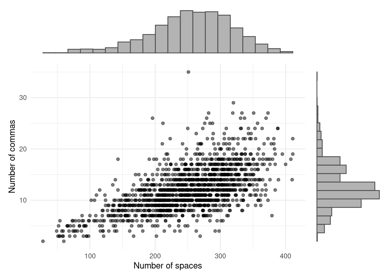
This example contains data on reviews published on Amazon. The dataset comprises information on 30 reviews by each of 50 reviewers, giving a total of \(n=1500\) reviews. For each review, a total of \(p=10,000\) variables are recorded, including word frequency (for example, the number of occurrences of the word ‘book’ in each review); usage of digits and punctuation; word and sentence length; and usage frequency of words and so on. A scatterplot of two of the variables (number of spaces in the review, and number of commas) appears in Figure 1.2, along with histograms displaying the marginal distributions of each variable.

Figure 1.2: Plot of number of commas against number of spaces in reviews on Amazon.
Perhaps the first thing that stands out in this example, compared to the last one, is the sheer quantity of data. Here there are 15 million individual pieces of data, whereas we had just \(120\) in the goats dataset. A second noteworthy point is that the dataset is massively multivariate. Classical statistical theory and methods (like linear regression, for example) are designed for cases where there are (many) more records (\(n\)) than variables (\(p\)), but we have quite the reverse for the Amazon data.
The Amazon review data were collated, in part, to provide the raw material for developing tools for authorship identification. In other words, given a particular new review by purported author X, is there an automated methodology by which we can examine whether it truly is by X by looking at earlier reviews by the same author? This is a classification problem (often referred to as a supervised learning problem by computer scientists). Of course, such a rich dataset can also be used to address other problems in stylometry3, natural language processing4 and linguistics. For example, one might look for associations in the use of written language. If someone typically writes in long sentences and uses many commas, are they also likely to be a relatively heavy user of semi-colons?
Such classification and association problems are common in data mining. Furthermore, the methods and models used to address them are usually highly complex and do not have easily interpretable parameters. This lack of interpretability is usually inconsequential to the data miner: the quality of a classifier, for example, being measured solely in terms of its ability to correctly assign individuals to the correct category.
Having explored some of the underlying ideas, we are now in a position to list some of the differences between classical statistics and data mining. As intimated above, the boundaries between these areas are somewhat fluid, so the distinctions that we draw are hardly set in stone. Nonetheless, they should provide you with a feel for what data mining is all about.
Data mining almost always involves large to massive datasets, while the datasets in classical statistical analyses can be quite modest in size. In this paper we focus principally on large datasets (say \(10^3\)–\(10^6\) elements) rather than massive ones, in order to allow you to perform analyses on your home computer.
Classical statistical methods are typically designed to deal with situations where there are many more records \(n\) than variables \(p\). In data mining the reverse will sometimes be true. An important modern instance of this occurs with gene expression data, were we typically have measurements on thousands of genes taken from tens to hundreds of people or specimens.
In classical statistics the aim of an analysis is often estimation or testing of some parameter or another. In data mining the problems are more often concerned with classification, prediction, or association. Sometimes a data miner will not have any specific aim beyond developing a better understanding of the data. In that case, data mining is very much an approach to exploratory data analysis.
Classical statistical models are usually easy to interpret; for example, one can write down the fitted model in a straightforward manner. In data mining the models are typically complex and ‘black box’ in nature.
1.2 Statistical Computing with R
This course makes heavy use of the statistics package R. You may have met this package before and be confident using it, in which case you will be aware how wonderful it is! If not, don’t worry. You’ll find an introduction to R in the second chapter of these notes, and plenty of guidance in its use throughout the remainder of the study guide.
For those of you who haven’t met R before, you’re in for some good news
– this package is freely available for download from the website
https://www.r-project.org/. Some even better news is that R is
state-of-the-art statistical computing, and is widely used package by
statistics researchers. It is extremely flexible and powerful.
Be warned, however, that R is not ‘point and click’. You need to type in commands. In fact this is a great thing from a learning perspective, since it requires you to think about what you are doing! While you may find R hard going to begin with, you will most likely be a fan of the package by the end of semester. That’s certainly our experience with the great majority of students. Nonetheless, it requires practice.
A crucial learning element of this course are the practical computing workshops. Not only do they allow you to practice what you’re learning, but they also teach you some techniques that will be useful for other courses.
1.3 The tidyverse
Our philosphy is to use the tidyverse as much as we practically can.
If you haven’t used the functionality in the tidyverse much in the
past, then we can recommend the online text “R for Data Science” by the author
of much of the tidyverse, Hadley Wickham:
In addition, the main tidyverse website is a useful resource:
Every student taking a 300-level statistics paper should be at least vaguely familiar with the names Ronald Fisher and Karl Pearson. Look them up on Wikipedia if you’re not!↩︎
To be a little more precise, we would use an analysis of covariance (ANCOVA) type of model, something that you can learn about in the paper 161.251 Regression Modelling.↩︎
Stylometry is the study of style to determine the origin of a work (linguistic style in the case of authorship of books, artistic style in the case of provenance of paintings, etc.).↩︎
Natural language processing is a branch of artificial intelligence concerned with computer handling of human language.↩︎