Chapter 3 Missing values
Dealing with missing values is a critical part of the data mining process. It is typical that variables in our data will be incomplete, where one (or often thousands) of observations may be missing that measure.
In some cases we may be able to fill in these gaps through judicious use of other variables for which the data are not missing. In other cases it may be best to discard variables or observations for which we have little data.
3.1 Patterns of Missingness
As noted in Section 2.4, it is not unusual for real datasets to contain missing values. We have already met some examples, with missing values present in the husbands and wives dataset.
The importance of the presence of missing values depends on a number of things. For example, how many data are missing, and what is the pattern of missing data values across the dataset? To address these questions, let us think about the probability that each entry in the dataset is missing. It might be that the data are missing completely at random (MCAR). By that, we mean that the probability of an entry being missing for some variable is equal across all records in the dataset. Alternatively, it could be that the probability of recording a missing value depends on the true (but unrecorded) data value. There is a further distinction that can then be drawn. On the one hand, it might be that the probability of missingness10 can be explained in terms of other variables where we do have data (in which case we say that the unavailable entries are missing at random (MAR). On the other hand, it could be that the probability of missingness is determined intrinsically by the true value of the missing datum, and that this probability cannot be explained in terms of the data that we do have11.
To illustrate these concepts, let us consider a geologist who is carrying large and heavy samples of crystals between labs. In the first lab the weight of each crystal is recorded, while in the second its volume is measured. The final dataset should include weight and volume for each sample, but some crystals are dropped and smash on the ground en route between the labs and therefore have missing values for volume. If the geologist is equally likely to fumble and drop any of the crystals, then the volume data will be missing completely at random. If instead, the geologist has a tendency to drop the heavier crystals, then the we would likely model the missing volume data as missing at random. However, it might be that it is the bulk rather than the weight of the crystals that makes them difficult to handle, in which case the probability of dropping each one will depend on its volume. The data are then not missing at random.
The situation where the data are not missing at random is particularly challenging. In many cases a thorough investigation of the processes involved in the pattern of missingness can be revealing. This might involve collection of further data or checking the data processing procedure. For example, it might transpire that true extreme values are rejected as measurement error and reported as missing values by automated data capture and processing software12. However, it is more common to assume that the pattern of missingness is either MCAR or (more commonly) MAR. Arguably, the significance of the missing data mechanism is more important when doing classical statistics (i.e. building statistical models, testing hypotheses and so forth). Nonetheless, it is worth keeping in mind that the conclusions drawn from any data mining procedure may be sensitive to the assumptions that we make about missing values.
3.2 Visualising missing values
It is useful to get an overview of where missing values are, as that may assist us in determining how to procede. For example, if almost all the missingness is confined to just one variable (column), removing that variable from subsequent analyses may be the way to go. Or, if missingness is instead confined to a small number of observations (rows) then removing those rows might be more appropriate. Or a combination thereof!
The vis_miss() function in the visdat package is useful for this.
Example 3.1 Visualising missingness in the airquality data
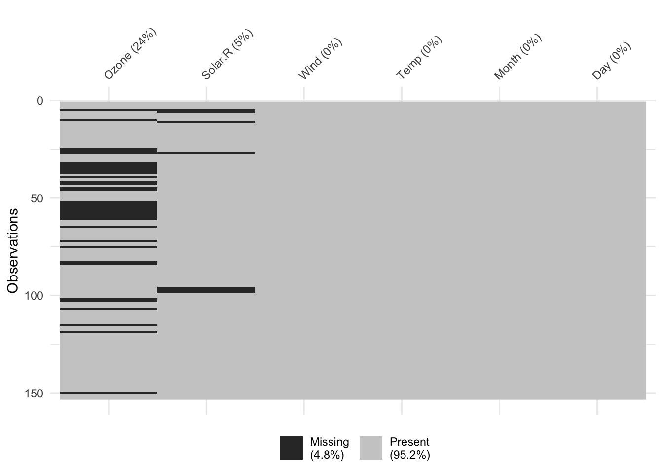
We can use vis_miss directly on the airquality data.frame:
 From this we see that most of the missingness (4.8% overall) is contained in the
 Ozone column,
which is 24.2% missing. The Solar.R column then contains relatively small number of missing rows (7)
while the other rows are complete. Depending on the analyses, it might be appropriate to remove
the Ozone variable before continuing on.
3.3 Working with Complete Cases
The impact that missing data will have on any subsequent analysis will
depend on the proportion of the data points that are missing (all other
things being equal). If there are just a few missing values, or if there
are missing values on many variables but restricted to a small number of
records (i.e. cases), then a simple way to deal with them is to exclude
all cases with missing values. In other words, we retain only complete
cases. This is simple to do in R using the complete.cases function.
Example 3.2 Deletion of Incomplete Records for the Husbands and Wives Data
Recall that the husbands and wives data contains 199 records, each corresponding to a husband-wife pair for which the following variables are recorded.
H.Age |
Husband’s current age (in years) |
H.Ht |
Husband’s height in millimetres |
W.Age |
Wife’s current age (in years) |
W.Ht |
Wife’s height in millimetres |
H.Age.Marriage |
Husband’s age (in years) when first married |
We processed these data earlier so that missing values are specified by
the usual NA convention in R.
Suppose that we wish to compute the correlation matrix for these data. This is a matrix with ones on the long-diagonal (corresponding to a perfect correlation of any variable with itself) and pair correlations as the off-diagonal elements13.
#>                     H.Age       H.Ht W.Age       W.Ht H.Age.Marriage
#> H.Age           1.0000000 -0.2773030    NA -0.2118564             NA
#> H.Ht           -0.2773030  1.0000000    NA  0.3644337             NA
#> W.Age                  NA         NA     1         NA             NA
#> W.Ht           -0.2118564  0.3644337    NA  1.0000000             NA
#> H.Age.Marriage         NA         NA    NA         NA              1
We see from this that there is a positive correlation of \(0.36\) between
wives’ and husbands’ heights (i.e. W.Ht and H.Ht), although it is
not particularly strong. However, much of the correlation structure in
the data is hidden from us because of missing values in the correlation
matrix. These occur because R returns NA when it tries to compute the
correlation between a pair of variables where either one contains
missing values.
One way of handling this is to delete all records which are incomplete (i.e. contain at least one missing value).
complete_rows <- complete.cases(husbands)
husbands2 <- husbands |> filter(complete_rows)
nrow(husbands2)
#> [1] 169#> H.Age H.Ht W.Age W.Ht H.Age.Marriage
#> H.Age 1.0000000 -0.2251498 0.9382382 -0.1931005 0.3624374
#> H.Ht -0.2251498 1.0000000 -0.1563196 0.3041247 -0.1032112
#> W.Age 0.9382382 -0.1563196 1.0000000 -0.2062793 0.2364224
#> W.Ht -0.1931005 0.3041247 -0.2062793 1.0000000 -0.0368114
#> H.Age.Marriage 0.3624374 -0.1032112 0.2364224 -0.0368114 1.0000000Points to note:
We start off with 199 records, which is the number of rows in the data frame (which can be found using the
nrowfunction).The command
complete.cases()returns a logical vector, withTRUEfor each row of the data frame which is a complete case (i.e. does not contain missing values) andFALSEfor incomplete cases.The
filter(complete_rows)command filters the data and returns only those rows wherecomplete_rowsisTRUE(i.e. only rows that are complete). The first two lines of code could alternatively be done using themagrittrpipe%>%viahusbands2 <- husbands %>% filter(complete.cases(.)). The special.argument here is specific to the%>%pipe and represents the data on the left of the pipe. The base R pipe as of R 4.2.0 doesn’t yet have this same capability.The complete case data frame has 169 rows, indicating that there were 30 (\(=199-169\)) incomplete records.
The correlation matrix for
husbands2has no missing values. As one might expect, by far the strongest correlation is between wives’ and husbands’ ages (W.AgeandH.Age).
3.4 Missing Data Imputation
In the previous example, deletion of the incomplete cases led to a relatively small reduction in the sample size: \(n=199\) down to \(n=169\). In such circumstances case deletion is a reasonable approach to handling missing values. However, suppose that we have a dataset with 100 variables, and a probability of 2% that each data item will be missing. In that situation only about 13% of the records would be complete, so that deleting incomplete records would result in a massive reduction in sample size.
In any event, throwing away good data (like the available entries in an incomplete record) is an anathema to a Statistician, whose job should be to squeeze all the available information from a dataset. Nonetheless, many statistical methods will only work with complete data (as we saw when trying to find the correlation matrix in the previous example). This suggests that we look at ways of filling in the missing values by plausible surrogates. This is called imputation in Statistics.
Perhaps the simplest possible approach to imputation is to use an average value for each missing data item. For a quantitative variable we would replace each missing value by the mean; for a categorical variable we would use the mode (i.e. the most frequently occurring category).
Example 3.3 Mean Imputation for Husbands and Wives Data
The husbands and wives dataset has missing values for the variables
W.Age (wife’s age) and H.Age.Marriage (husband’s age when married).
The following R code replaces missing values by the variable mean for
the first of these variables .
library(naniar)
HusWife <- husbands |>
  mutate(W.Age.New = impute_mean(W.Age),
         H.Age.Marriage.New = impute_mean(H.Age.Marriage))
HusWife |> filter(is.na(H.Age.Marriage))
#> # A tibble: 4 × 7
#> H.Age H.Ht W.Age W.Ht H.Age.Marriage W.Age.New H.Age.Marriage.New
#> <dbl> <dbl> <dbl> <dbl> <dbl> <dbl> <dbl>
#> 1 46 1823 NA 1591 NA 40.682 25.364
#> 2 54 1679 53 1560 NA 53 25.364
#> 3 27 1765 NA 1571 NA 40.682 25.364
#> 4 32 1764 NA 1662 NA 40.682 25.364Points to note:
We start by loading the
naniarpackage which is useful for dealing with missing values in atidyverse-centric way.The
mutate()command then creates two new columns (with.Newappended), using theimpute_mean()function to do the imputation.Alternatively, we could have used
husbands |> impute_mean_all()to do this same operation - it will impute all missing values from every column using the mean of the remaining data.
Mean imputation ignores the correlation structure in the data, in the
sense that the imputed values do not depend on data on the other
variables. As a result, mean imputation can distort trends in the
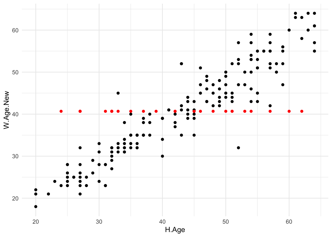
dataset. As an illustration, Figure 3.1
displays a scatterplot of wife’s age against husband’s age using the
imputed data set (HusWife), where the imputed values are coloured red.
Obviously the imputed values muddle what is otherwise a rather clear
trend between the two variables.

Figure 3.1: Scatterplot of wife’s age against husband’s age for the mean imputed dataset. Imputed values are coloured red.
A more plausible approach to imputation (for numerical variables) is to replace each missing value by a typical value based on similar records. For example, consider imputing the age of a wife with a 25 year old husband. We might approach this by looking at all complete cases with husbands that are around 25 years old (say in the range 22-28) and compute the ages of their wives. The mean of these values would likely be a far better reconstruction of the missing value than the overall mean of wives’ ages (which is 40.7 years).
To put this in practice we need to be precise about what we mean by
‘similar records’ in the above paragraph. If the data are numerical,
then we can measure similarity (or rather dissimilarity) by the distance
between records. There are various metrics that we could use, such
as the Euclidean distance 14. In practice, we’ll be using
Gower’s distance which is more stable than Euclidean distance, as
it first divides the values in each variable by the range, prior to computing
the Manhattan, or absolute distance15. If we have non-numeric
data then it uses simple matching. For a record with a missing value on some
given variable, we can then find the \(k\) nearest complete
cases (using Gower’s distance based on the variables for which we do
have data). The median of the variable in question for these \(k\) near
neighbours can then be used as a replacement for the missing value.
This methodology is known as k nearest neighbour imputation. It is
implemented in R using the kNN function from the VIM package.
In practice we must choose a value for \(k\). The crux of the issue is as follows. If we choose a small \(k\) then the imputed value will be somewhat unstable, being the mean of just a few values. Nonetheless, the values that we will be averaging over will all be quite like the incomplete case under investigation, since we are dealing with only very near neighbours. On the other hand, if we choose a large value of \(k\) then the imputed value should be much more stable (being the mean of many data) but we will incorporate information from some cases that are quite distant from (and hence quite unlike) the record in question. There are a number of sophisticated automated methods for choosing \(k\), but for in many cases \(k=5\) is a reasonable rule-of-thumb to use.
Example 3.4 \(k\) Nearest Neighbour Imputation for the Husbands and WivesData
In this example we impute values for the missing data on W.Age and
H.Age.Marriage using k nearest neighbour imputation.
Points to note:
The
library(VIM)command is loading theVIMlibrary.The
kNN()command does the imputation - by default it will impute using all columns. By default it will also return additional columns named<column_name>_impwhich states whether the values in that column were imputed.

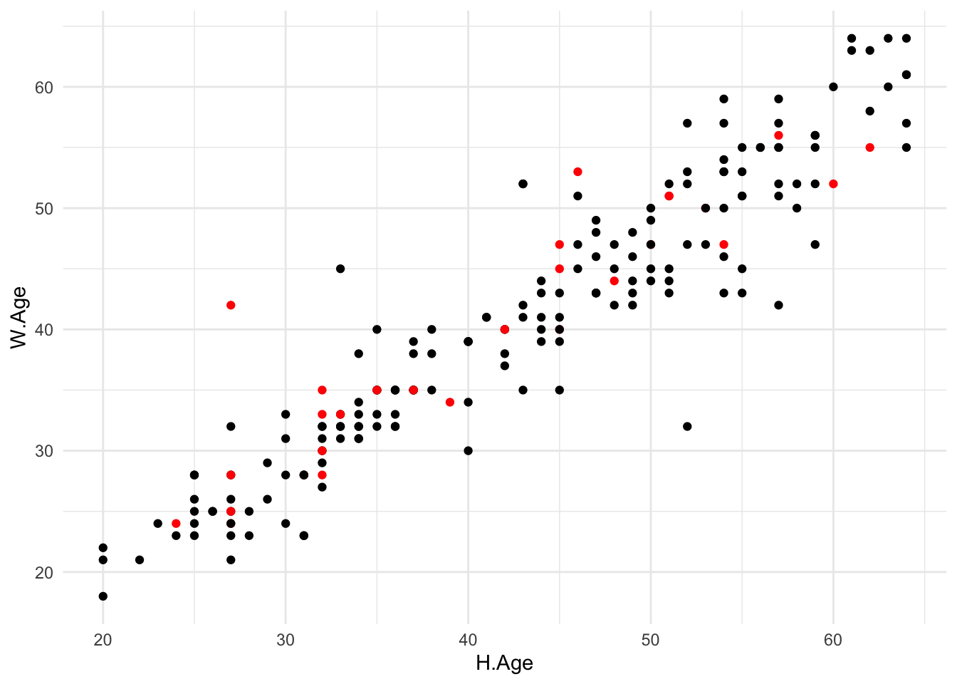
Figure 3.2: Scatterplot of wife’s age against husband’s age for the k nearest neighbour imputed dataset using \(k=5\). Imputed values are coloured red.
Finally, Figure 3.2 displays scatterplots of wife’s age against husband’s age using the imputed data set just created. As before, the imputed values are coloured red. It is clear that k nearest neighbour imputation does a far better job than mean imputation for this dataset.
3.5 Alternative Methods of Imputation
There are alternatives to mean imputation and k-nearest neighbour imputation. For example, regression based imputation applies (linear) regression models in order to predict the missing values based on the available data.
An important distinction is between single and multiple methods of imputation. We have focused solely on the former, where each missing value is replaced by a single imputation. A general problem with this approach is that we lose the sense of uncertainty in the imputed values. If we employ the resulting imputed dataset as if it were truly observed, then we are pretending that we have more information than is actually the case. It follows that the result from any analysis based on the imputed dataset will produce results which appear more precise than they should.
In multiple imputation we simulate multiple possible values for each missing data item. The idea is that this captures the sense of uncertainty in the imputed values. However, we are left with a somewhat complex data structure, where the original data are augmented by a raft of alternatives for each missing value. It follows that the use of multiply imputed datasets in subsequent analyses is not entirely straightforward.
While interesting, the details of these alternative methods of imputation are beyond the scope of this course.
If you were wondering, ‘missingness’ is a real word! It appears uncommon in everyday usage (it does not appear in my 1876 page Shorter Oxford English Dictionary, although it is in the full OED) but is very much part of the technical vocabulary of missing data analysis.↩︎
The descriptions of MCAR and MAR that we have given are not formal definitions. These concepts can be defined in an precise mathematical way, although this requires that we have some statistical models for the data, and in particular for the probability of missingness.↩︎
Circumstances rather like this have been credited for the delay in detection of the hole in the Antarctic ozone layer, where readings of almost zero ozone concentrations were flagged as unreliable by the data processing software and hence interpreted as ‘missing values’ by some scientists↩︎
Correlation is symmetric: that is, the \({\textsf {cor}}(X,Y) = {\textsf {cor}}(Y,X)\). As a consequence correlation matrices are symmetric.↩︎
Euclidean distance is the distance between points as measured by a ruler. By Pythagoras theorem, the Euclidean distance between the \(i\)th and \(j\)th records is defined by \[d_{ij} = \sqrt{ \sum_{\ell=1}^p (x_{i\ell} - x_{j\ell})^2 }\] where \(x_{i\ell}\) is the value of the \(\ell\)th variable for the \(i\)th case.↩︎
Manhattan distance is the distance between points as if you were in downtown Manhattan, so that you can only walk along the grid (horizontal or vertical). The Manhattan distance between the \(i\)th and \(j\)th records is defined by \[d_{ij} = \sum_{\ell=1}^p |x_{i\ell} - x_{j\ell}|\] where \(x_{i\ell}\) is the value of the \(\ell\)th variable for the \(i\)th case, and \(|x|\) denotes the absolute value of \(x\).↩︎